thunder4d.diagnostics

All functions take grid and a field Aw in \((x, y, \Omega)\) (FFT order) and return sorted axes. Wavelength-resolved densities are per unit wavelength unless per_lambda=False.

Basic quantities

thunder4d.diagnostics.spectral_support(grid, Aw, rel=1e-4)

Indices of the frequencies carrying more than rel × the peak spectral energy.

thunder4d.diagnostics.total_spectrum(grid, Aw, per_lambda=True)

Returns:

(lam, S), spatially integrated spectrum, ascending wavelength

thunder4d.diagnostics.fluence(grid, Aw)

Returns:

\(F(x, y)\) [J/m²]

thunder4d.diagnostics.temporal_power(grid, Aw)

Returns:

(t, P), spatially integrated power [W]

Near field and far field

Note

Far field = the cell centre (focus / waist plane): the plane where the field is stored, so profiles_1d(), spectrogram_x_lambda(), … describe the far field. Near field = the collimated beam, i.e. the angular spectrum of the cell-centre field (\(x_\text{out} = f\,\theta\) after a collimating lens of focal length \(f\)): near_field(), near_profiles_1d() and spectrogram_theta_lambda().

thunder4d.diagnostics.near_field(grid, Aw, theta_max=None, n_theta=None, idx=None, theta_y=None)

Angular spectrum \(E(\theta_x, \theta_y, \Omega)\) on an angle grid common to all colours, computed exactly with a per-colour matrix Fourier transform. This is what is seen after collimating the output with a lens of focal length \(f\), at \(x = f\theta\).

Parameters:

• theta_max (float) – default: half the largest \(k_x\) at \(\lambda_0\)

• n_theta (int) – default: an odd number, so \(\theta = 0\) is sampled

• theta_y – restrict to given \(\theta_y\) values, e.g. [0.]

Returns:

(theta_x, Ef), Ef of shape (n_theta, len(theta_y), Nt)

Spatio-spectral traces

thunder4d.diagnostics.spectrogram_x_lambda(grid, Aw, y0=0.0, slit=None, axis='x', per_lambda=True)

Imaging-spectrometer trace along a line, optionally integrated over a slit of width slit around y0.

Returns:

(x, lam, S[x, lam])

thunder4d.diagnostics.spectrogram_theta_lambda(grid, Aw, theta_max=None, n_theta=None, per_lambda=True)

Angle-resolved spectrum at \(\theta_y = 0\).

Returns:

(theta, lam, S[theta, lam])

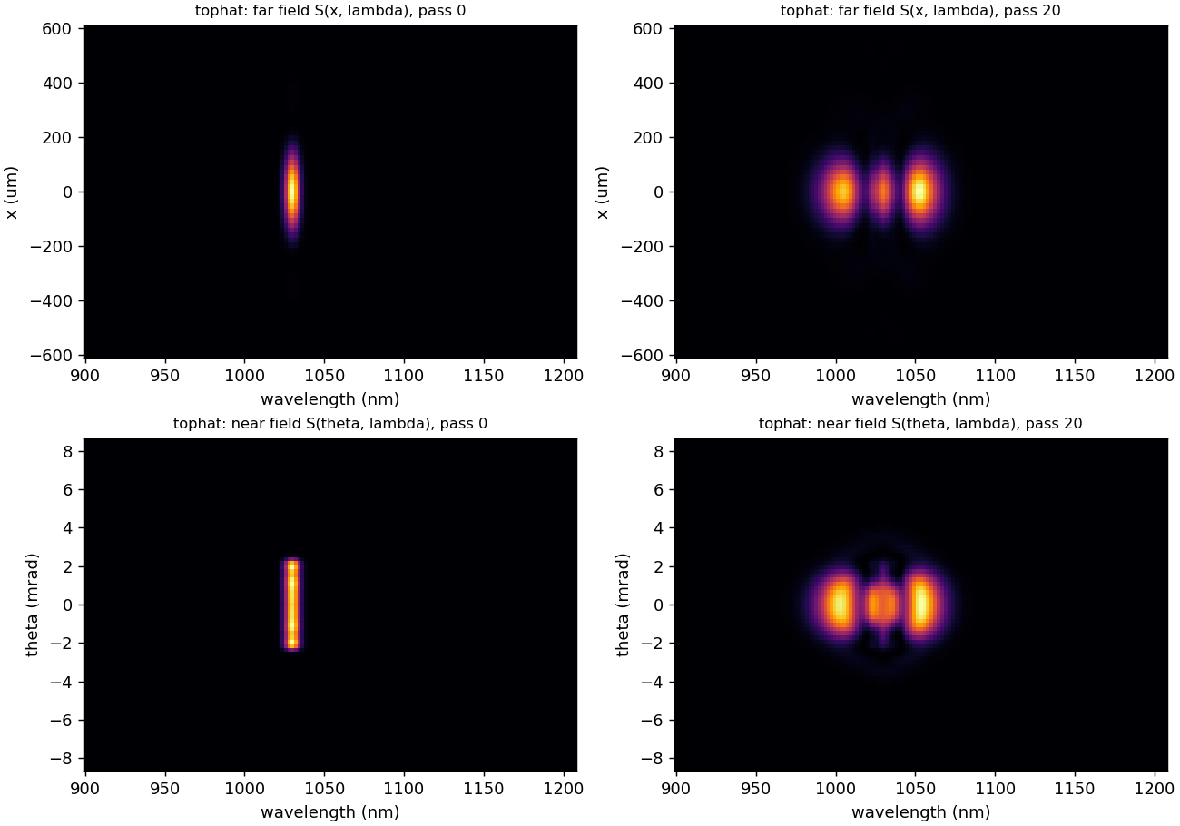
Fig. 9 \(S(x,\lambda)\) (top) and \(S(\theta,\lambda)\) (bottom), input and output.

Wavelength-resolved profiles

thunder4d.diagnostics.band_indices(grid, lam_c, bandwidth=0.0)

Frequency indices inside \([\lambda_c - bw/2, \lambda_c + bw/2]\) (nearest bin if bandwidth = 0).

thunder4d.diagnostics.profiles_1d(grid, Aw, wavelengths, bandwidth=0.0, axis='x', mode='cut')

1D beam profiles of selected wavelength bands plus the global (spectrally integrated) profile.

Parameters:

mode (str) – "cut" (line through the axis) or "integrated" (projection, like a 1D camera lineout)

Returns:

(coord, profiles[n_lambda+1, N], band_energy[n_lambda+1]); the last row / entry is the global profile / total energy [J]

thunder4d.diagnostics.near_profiles_1d(grid, Aw, wavelengths, bandwidth=0.0, theta_max=None, n_theta=None)

Same in the near field (collimated beam), cut at \(\theta_y = 0\).

Returns:

(theta, profiles[n_lambda+1, n_theta])

Homogeneity

thunder4d.diagnostics.homogeneity(grid, Aw=None, S_xyw=None, rel=1e-3)

Spectral homogeneity of each pixel against the total spectrum \(S_0\):

\[V(x, y) = \frac{\left(\sum_\lambda \sqrt{S(x,y,\lambda)\,S_0(\lambda)}\right)^2} {\sum_\lambda S \;\sum_\lambda S_0}.\]

\(V = 1\) is perfectly homogeneous. Pixels below rel × the peak fluence are NaN. Instead of a field, an intensity cube S_xyw can be given, e.g. abs(Ef)**2 from near_field(), for the near-field (collimated beam) homogeneity.

Returns:

(V_map, V_mean), V_mean fluence-weighted

Modal content

thunder4d.diagnostics.mode_content(grid, Aw, w0_of_lambda, max_order=6, idx=None)

Hermite–Gauss decomposition, frequency by frequency, on modes of waist w0_of_lambda(lam) with a flat phase (exact at the cell centre).

Returns:

dict with lam, eta00 (HG₀₀ fraction per wavelength), eta00_total, order_frac (energy fraction per order \(m+n\); the last bin holds everything above max_order)

Beam size and beam quality

thunder4d.diagnostics.lg_mode_content(grid, Aw, w0_of_lambda, p_max=2, l_max=2, idx=None)

Decomposition on Laguerre-Gauss modes \(\mathrm{LG}_{pl}\) (\(e^{il\varphi}\) convention, waist w0_of_lambda(lam), flat phase), spectrally integrated. Returns p (\(0..p_{max}\)), l (\(-l_{max}..l_{max}\)), frac[p, l] (fraction of the total energy per mode) and residual (energy outside the listed modes).

thunder4d.diagnostics.beam_moments(grid, Aw, idx=None)

Per wavelength: second-moment radii wx, wy [m] and M2x, M2y from the Wigner moments \(M^2 = 2\sqrt{\langle x^2\rangle\langle k_x^2\rangle - \langle x k_x\rangle^2}\) (centroids removed). Also returns lam and the spectrally weighted M2x_mean, M2y_mean.

Note

Second-moment quantities are sensitive to far wings: hard edges and Airy rings inflate \(M^2\).

Compression and chirp maps

thunder4d.diagnostics.compress(grid, Aw, gdd_bounds_fs2=(-30000, 30000), tod_fs3=0.0, n_scan=61, rel=1e-4)

Uniform GDD (e.g. chirped mirrors) maximising the peak of the spatially integrated power: coarse scan, then golden-section refinement. tod_fs3 adds a fixed TOD.

Returns:

dict with gdd_fs2, t_fs, P (compressed \(P(t)\) [W]), fwhm_fs, tl_fwhm_fs (spatially resolved transform limit), peak_power, peak_power_TL, gdd_scan_fs2, peak_scan

thunder4d.diagnostics.local_gdd_map(grid, Aw, rel_fluence=1e-2, rel_spectrum=1e-2)

Pixel-wise GDD [fs²] from a spectrally weighted quadratic fit of the unwrapped spectral phase (radial chirp). NaN outside the beam.

thunder4d.diagnostics.radial_profile(grid, M2d, nbins=None)

Azimuthal average of a sorted 2D map.

Returns:

(r, value)