Design helper

thunder4d.design goes from a laser and a target to ranked, ready-to-run cells: gas, pressure, radius of curvature, round trips and passes, with the margin to every limit. It works in three layers:

Layer	Per cell	Use
analytic estimates	microseconds	discard geometries, rank starting points, draw maps
fast1d (1+1D)	0.1–0.2 s	rank, tune and check the candidates
thunder4d (4D)	seconds to minutes	simulate the design you keep

The notebook examples/design_tutorial.ipynb is the interactive version of this page; the graphical interface has a panel for it. The plots need matplotlib (thunder4d[examples]).

Example

18 mJ, 500 fs at 1030 nm, to be compressed to 25 fs in argon or krypton:

from thunder4d.design import DesignProblem, Fast1DQuick, LaserSpec, Max, MPCDesigner, Target, starting_points

problem = DesignProblem(
    laser=LaserSpec(energy_J=18e-3, duration_fs=500.0, rep_rate_Hz=1e3),
    target=Target(objective="target_duration", target_duration_fs=25.0),
)
C = problem.constraints
C.space.max_separation_m.value = 5.0                 # m
C.mirrors.allowed_roc_m = (1.0, 2.0, 3.0)            # the mirrors you can use
C.mirrors.fluence.value = 0.7                        # J/cm² (None: LIDT of the coating)
C.kerr.b_per_pass_rad.value = 3.0                    # rad, on axis
C.ionization.peak_intensity_W_cm2 = Max(3.5e13)      # W/cm²
C.gas.allowed = ("Ar", "Kr")
problem.search.round_trips = (8, 25)
problem.search.branches = ("concentric",)
problem.refinement.n_candidates = 3

if __name__ == "__main__":                           # needed on Windows with workers > 1
    result = MPCDesigner(problem, quick=Fast1DQuick(), workers=4).refine(starting_points(problem))
    print(result.table())
    print(result.best.report(problem))
    result.export("design.json")                     # standard input file

 #  gas  p[bar]  R[m]   M   k    N     branch   d[m]  tau[fs]     T    score
 0   Ar   0.170  2.00  15   2   29 concentric  3.827     25.4 0.986  0.00924
 1   Kr   0.050  2.00  17   3   34 concentric  3.700     27.9 0.983   0.0215
 2   Ar   0.110  3.00  25   7   50 concentric  4.912     29.6 0.975   0.0365

Ar 0.170 bar | R = 2.0 m, M = 15 round trips, k = 2, concentric, d = 3.827 m, 29 passes | dielectric_1030nm, 3"
  output : 25.4 fs (from 500 fs, x19.7), throughput 98.6 %, peak power 435 GW
  score  : 0.00924  = objective 0.000229 + penalties 0.00901   (lower is better)
  limit                    value           limit   margin  mode
  main_peak               0.6335  >=         0.7      -9%  soft  <-- violated
  fluence [J/cm2]         0.5582  <=         0.7      20%  hard
  b_per_pass [rad]         2.342  <=           3      22%  hard
  throughput              0.9856  >=         0.8      23%  soft
  separation [m]           3.827  <=           5      23%  hard
  ionization [W/cm2]   2.416e+13  <=     3.5e+13      31%  hard
  p_over_pcr              0.3405  <=         0.5      32%  hard
  pressure [bar]            0.17  <=           3      94%  hard
  bandwidth            7.976e-05  <=        0.01      99%  hard
  spot_separation [w]       7.941  >=           3     165%  hard
  spots  : 15 per mirror on r = 33.7 mm, 7.9 w apart
  align  : d +- 1 mm -> w0 0.1 %, w_mirror 0.2 % | RoC +- 0.5 % -> w0 3.0 %, w_mirror 2.9 %

The best design is argon at 170 mbar, \(R = 2\) m, 15 round trips, \(k = 2\), 29 passes. Its only violated limit is soft: 63 % of the energy in the main peak for a floor of 70 %, the pedestal of a broad spectrum compressed with GDD only. The report lists the limits from the tightest to the loosest: the first line is what constrains the design.

The problem

DesignProblem has seven blocks, all dataclasses with defaults; set only what matters.

Block	Content
laser	energy, duration, wavelength, transform limit if chirped, shape, pre-chirp, repetition rate, polarisation. LaserSpec.preset("pharos_ph2_sp_2mJ", rep_rate_Hz=1e3) takes a datasheet.
target	objective: "max_peak_power" (default), "shortest", "target_duration", "target_compression" or "weighted"; soft floors min_throughput (0.8) and min_main_peak_fraction (0.7)
constraints	space (max_separation_m 4 m), mirrors (radii, diameters, coatings, fluence, bandwidth), Kerr (p_over_pcr 0.5, b_per_pass_rad 1 rad), ionisation, spot pattern (spots 3 radii apart, 2.5 radii from the edge), pressure range (0–3 bar) and resolution, gases
losses	mode_matching_efficiency
search	which geometries are tried: gases, radii, branches, round trips \(M\) (3–40), \(k\), passes per geometry
refinement	how many designs (5), what is tuned (pressure, optionally the pre-chirp), neighbours tried
tolerance	alignment errors whose effect each report gives (information only)

A Herriott geometry is \((R, M, k)\), with \(d = R\,(1 \pm \cos(\pi k/M))\) (+: concentric). One cycle is \(2M\) passes with \(M\) spots per mirror; the passes used can be fewer.

Limits. Every constraint is a Limit, built with Max(...), Min(...) or Off(). mode="hard" rejects a design that violates it, "soft" adds weight * margin**2 to the score. value=None takes the value from the catalogue (LIDT of the coating at the pulse duration of each bounce, ionisation threshold of the gas). The limit applied is value * safety for a maximum.

Warning

Setting only .value keeps the safety in place: the ionisation limit has safety = 0.5, so peak_intensity_W_cm2.value = 3.5e13 applies 1.75e13 W/cm². Replace the whole limit (Max(3.5e13)) to reset it.

Catalogues. The gases take their dispersion and \(n_2\) from thunder4d.materials and add an ionisation threshold, by default 0.2 times the barrier-suppression intensity: an order of magnitude, set your own. The mirror catalogue has three coatings (dielectric_1030nm, dielectric_800nm, enhanced_silver); add yours:

from thunder4d.design.catalog import GASES, Coating, register_mirror

GASES["Ar"] = GASES["Ar"].with_(ionization_threshold_W_cm2=4e13)
register_mirror(Coating.from_files("my_hr", "R.csv", "GDD.csv", delimiter=",",   # columns: nm, value
                                   lidt_J_cm2=0.7, band_nm=(950.0, 1110.0)))

The search

starting_points()  ->  screen()  ->  refine()
enumerate and          rank with the       run the quick solver, tune the
prefilter              analytic estimates  best candidates, return n designs

• starting_points enumerates the allowed geometries and drops those that a hard limit already excludes analytically (separation, fluence, ionisation, spot pattern). It never drops a cell that could pass. Each one starts at an analytic guess of the pressure.

• screen ranks them with the analytic estimates and keeps the best, spread over gases, radii and branches. refine runs the quick solver on them, tries their neighbours (more or fewer passes, next radius), optimises the pressure and rounds it to your regulator.

• The score is the objective plus the penalties of the soft limits; a violated hard limit makes it infinite. Ask for several designs: the first ranking uses the untuned pressure.

• MPCDesigner(..., workers=N) runs the quick solver in N processes.

Quick solvers

A quick solver is any callable quick(problem, candidate) -> QuickResult; only the duration, the peak power and the throughput are required, every other field is checked against its limit.

• AnalyticQuick: closed forms, no dispersion. Its durations are optimistic: use it to explore, not to decide.

• Fast1DQuick: a time envelope with the full dispersion of the gas, coupled to a Gaussian beam followed through its \(q\) parameter (thin Kerr lens at each step), with the mirror curves of the coating at each bounce. accuracy="fast" (0.1–0.2 s) is within 0.4 % of "fine" (2–8 s). It stops on beam collapse, optical shock or runaway step counts, and the cell is then rejected.

fast1d is least reliable when \(P/P_c\) is not small (its Gaussian ansatz is the weak point), for very broad spectra, and for non-Gaussian, clipped or mismatched beams. Treat its durations as good to a few percent on moderate cells and about 10 % on strongly nonlinear ones. Fast1DQuick().validate(problem, design) checks that it is converged for a design.

Maps

A map shows, for two parameters, where a cell is feasible and, where it is not, which limit excludes it: the fastest way to see what limits a design.

import numpy as np
from thunder4d.design import design_map

m = design_map(problem, gas="Ar", roc_m=2.0, k=2)                    # pressure × round trips, analytic
m.plot(mark=[(0.17, 15, "reference cell")])
m = design_map(problem, gas="Ar", roc_m=2.0, k=2, quick=Fast1DQuick(), workers=8)
design_map(problem, gas="Ar", roc_m=2.0, k=2, round_trips=15,
           x=("energy_J", np.linspace(5e-3, 30e-3, 12)), y=("pressure_bar", np.linspace(0.05, 0.3, 12)))

Axes: pressure_bar, round_trips, n_passes, roc_m, k, energy_J, duration_fs. The result keeps the limiting constraint, the tightest margin and the metrics at every point.

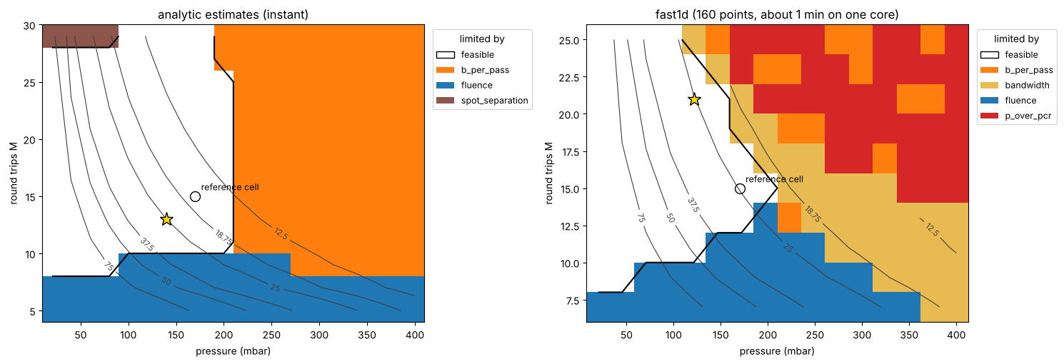
Fig. 2 Argon, \(R = 2\) m, \(k = 2\). Left: analytic (0.3 s). Right: fast1d (160 points, one minute). White is feasible; each colour is the limit that excludes the region; grey lines are the compressed duration in fs.

From a design to the 4D solver

A design is exported as a standard input file and runs with nothing from the helper:

import thunder4d as th

result.export("design.json", preset="medium")      # or to_input(problem, candidate) for a dict
b = th.run_input("design.json")

preset sets the grid ("coarse": seconds to minutes, "medium", "fine": benchmark grade), injection the beam (linear or Kerr-matched eigenmode), and the spectral window follows the predicted spectrum. The file records the predictions and margins in its design block.

validate_4d(problem, design) runs fast1d and the 4D solver on the same cell and compares them. On the example design, coarse grid, 9 s:

quantity                        fast1d          4D     diff
transmission                    0.9856      0.9757    -1.0%
B-integral [rad]                 63.23       67.95    +7.5%
compressed duration [fs]         25.34       24.79    -2.2%
compressed peak [GW]             435.3         403    -7.4%
mirror fluence [J/cm2]          0.5587      0.5139    -8.0%
M2 (x, mean)                                 1.002

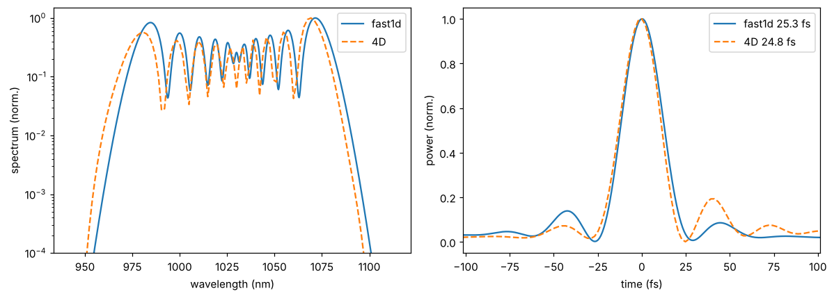
Fig. 3 Output spectrum and compressed pulse of both solvers on the example design.

The durations and the transmission agree within a few percent. At \(P/P_c = 0.34\) the beam is no longer a perfect Gaussian, so the 4D B-integral is higher and the peak power and fluence lower: when a margin matters, use the 4D numbers.

Workflow. Search with fast1d and keep three to five designs; check fast1d’s convergence on each; validate_4d each; export the one you build at "medium" or "fine", edit the file (measured spectrum, injection) and run it.

Scope. One stage, an ideal GDD compressor, a Gaussian beam, no Raman (N₂ and air are flagged), no ionisation loss (the intensity is limited, not simulated). The margins are only as good as the thresholds you give.